If you want to learn Excel – or improve your existing skills – but not sure how to get started and what features you should definitely know about, fret not.
In this article, I’m going to talk about 12 aspects of Microsoft Excel which not everyone may be aware of but which I think are essential to all users in order to get the most out of the software. Most of these are quite easy to learn and use, but their benefits could be quite dramatic.
Absolute references
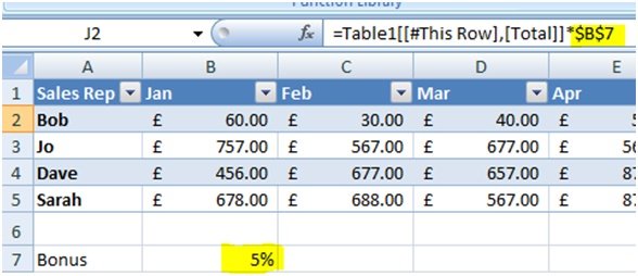
There are two types of references in Excel – absolute and relative references – and funnily enough, most Excel users use the latter without even knowing they are doing it.Relative referencing is the process of creating a formula and then using the auto fill function to apply this to other cells close by.
There may be times, however, when you don’t want a cell reference to change when filling in cells, such as a cell with a specific rate to which all formulas must reference and adhere to.

In this case, you would use absolute references which, unlike relative ones, don’t change when they are copied or filled in.
Using tables
The word “table” has slightly different meanings across all Microsoft Office applications.In Word, it is more to do with controlling the layout of titles, words and sentences, while in Access we use them specifically to organise data – in Microsoft Excel, however, it is a bit of both.

At first glance, tables in Excel provide the user with a nicely laid out set of columns with built-in filters.However, when a table is created, the table and its fields become referable the same way as anything in the name manager. This means that if you name your table and fields correctly, you can use structured references from anywhere within your workbook to its fields, i.e.
=count(Tablename[fieldname])
If the data on your spreadsheet is going to contain many rows of data, it is, in my opinion, a no brainer to format it as a table – but always make sure to name the table accordingly.
Creating dynamic charts from tables
Have you ever created a chart and worked really hard at formatting it, only to realise that you have to go back and update its references every time a new row of data isadded?
Another reason for using tables is that if you’ve formatted the data as a table before creating the chart(you can do this by simply highlighting the table’s required fields and inserting the chart), the chart is going to be dynamically linked to the table – meaning that whenever you add or delete rows, the table will automatically update itself.
If you need a step-by-step guide for this, Tech Republic has a great article on the topic.
Using the status bar
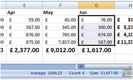
One of the easiest yet most handy tools in Excel is the status bar. The status bar is situated at the bottom right of the Excel window, and its function is to display the current sum, the average, the minimum and the maximum values of the cells selected.It is a quick but very effective reference tool which, with little fuss, can be customised to show or even hide various other functions.

Switching to formula view
There may be times when you want to revise all the formulas you used on your spreadsheet,butselecting the cell then viewing the formula in the formula bar can become a bit tedious and frustrating after a while.
Excel has had, for as long as I can remember, the option to alter the view to “formula view”, where each cell displays the formula rather than the actual result it calculates.It’s a simple click of a button in the Formulas tab to switch it on and off again and, as an added bonus, formula view will also let you print all your formulas in one go.

Rounding numbers
Sometimes you will create a formula which returns numbers with lots of decimal places,but you only want a few.Excel has many different ways of rounding numbers, from simply formatting a cell to specify how many decimal places you need to applying simple rounding functions to round up or down. All of these techniques are worth learning for any intermediate Excel user working with figures.
Scale to fit your printout to one page
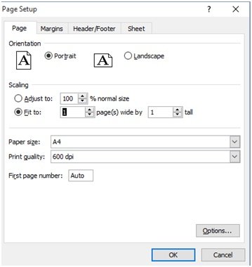
Excel can be a nightmare to print. Unlike Word, which works to A4 paper or any other size you specify, Excel spreadsheets are not uniform in size and can be very tall, wide or both.
Printing in Excel is more like a survival guide than an absolute science so, understanding the “scale to fit” settings in the Print Options menu is a great place to start to help get your spreadsheet to behave when you are printing it.

Using pivot tables
Pivot tables (and charts) are an excellent and quick way of summarising vast amounts of data on a spreadsheet – and, if the spreadsheet has been set up properly to start with, they are quite easy to use as well.By simply using drag and drop techniques, you as the user can easily have questions about your data answered in a few clicks.
“How have car sales in Spain been last month?”
Click, click, and you’re there.
“How is Bob getting on this month?”
Click, click, done.
And the best thing is, you don’t even need fancy “IF statements” or other functions for the most of it.
Using sparklines
Although charts are useful for displaying your data visually and helping you identify certain trends, they are usually quite big in size and are often displayed on separate worksheets, making it more difficult for you to go back to the actual data to view the figures for fine tuning. And this is when sparklines can help you.

Sparklines provide so-called “mini charts”, which fit into a cell and are there to simply accompany your data and quickly give you trend patterns without getting in the way. They are not as detailed as charts, of course, but are an excellent addition to support large, data-intensive spreadsheets and can make trends much quicker to identify.
Conditional formatting
If you’re working with a large number of data, your spreadsheet can easily become a sea of figures, making it very hard for you to identify particular values. Conditional Formatting is an excellent set of tools which you can apply to a cell or range of cells to highlight values if they fall within a specific criteria.
For example,in the picture below, all cells which have a value of less than £50 have been formatted with a redfill and bold text, whereas all cells which have a value greater than £300 have a green fill and bold text.

Finding circular references
Occasionally, you may encounter the circular reference error in Excel when opening a workbook.A circular reference is when a formula refers to itself, which could cause a knock-on effect – unfortunately, however, when the error appears it doesn’t tell you what cell or cells it applies to.

Circular references can be located quite easily, however, by using the Error Checking option in the Formula Auditing group of options. This will pinpoint the cell the error is in for a closer analysis.
Removing duplicates
Whether you use Excel on a daily basis or just occasionally, you will come across duplicated rows of data in your spreadsheets from time to time.The good news isthat the “Remove Duplicates” option enables you to instruct Excel to compare specific columns in a spreadsheet and remove duplicates as specified.
However, you need to be very careful with this. If done properly, it could save you hours of time filtering and sifting through massive data sets for duplicates, but in the wrong hands it could remove data you want to keep.
So, I hope the tips given in this article were helpful, and will allow you to become more productive using Excel. If you would like to expand your knowledge further, fortunately there are plenty of great resources and training courses out there. You can find details of Excel training courses on the Activia website, as well as tutorials and articles that will help you to use the software better.
Can you think of any other features that you think are important to know in Excel? Let us know in the comments below.
